MARKOV CHAINS:ABSORBING STATES

ABSORBING STATES

It was pointed out in Sec. 29.4 that a state k is called an absorbing state if pkk = 1, so that once the chain visits k it remains there forever. If k is an absorbing state, and the process starts in state i, the probability of ever going to state k is called the probability of absorption into state k, given that the system started in state i. This probability is de- noted by fik.

When there are two or more absorbing states in a Markov chain, and it is evident that the process will be absorbed into one of these states, it is desirable to find these probabilities of absorption. These probabilities can be obtained by solving a system of linear equations that considers all the possibilities for the first transition and then, given the first transition, considers the conditional probability of absorption into state k. In particular, if the state k is an absorbing state, then the set of absorption probabilities fik satisfies the system of equations

Absorption probabilities are important in random walks. A random walk is a Markov chain with the property that if the system is in a state i, then in a single transition the sys- tem either remains at i or moves to one of the two states immediately adjacent to i. For example, a random walk often is used as a model for situations involving gambling.

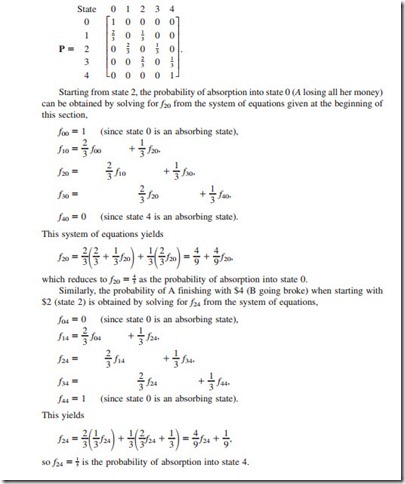
A Second Gambling Example. To illustrate the use of absorption probabilities in a random walk, consider a gambling example similar to that presented in Sec. 29.2. However, suppose now that two players (A and B), each having $2, agree to keep playing the game and betting $1 at a time until one player is broke. The probability of A winning a single bet is --, so B wins the bet with probability --. The number of dollars that player A has before each bet (0, 1, 2, 3, or 4) provides the states of a Markov chain with transition matrix

A Credit Evaluation Example. There are many other situations where absorbing states play an important role. Consider a department store that classifies the balance of a customer’s bill as fully paid (state 0), 1 to 30 days in arrears (state 1), 31 to 60 days in arrears (state 2), or bad debt (state 3). The accounts are checked monthly to determine the state of each customer. In general, credit is not extended and customers are expected to pay their bills promptly. Occasionally, customers miss the deadline for paying their bill. If this occurs when the balance is within 30 days in arrears, the store views the customer as being in state 1. If this occurs when the balance is between 31 and 60 days in arrears, the store views the customer as being in state 2. Customers that are more than 60 days in arrears are put into the bad-debt category (state 3), and then bills are sent to a collection agency.

After examining data over the past several years on the month by month progression of individual customers from state to state, the store has developed the following transition matrix:4

Although each customer ends up in state 0 or 3, the store is interested in determining the probability that a customer will end up as a bad debt given that the account belongs to the 1 to 30 days in arrears state, and similarly, given that the account belongs to the 31 to 60 days in arrears state.

To obtain this information, the set of equations presented at the beginning of this section must be solved to obtain f13 and f23. By substituting, the following two equations are obtained:

4Customers who are fully paid (in state 0) and then subsequently fall into arrears on new purchases are viewed as “new” customers who start in state 1.

Thus, approximately 3 percent of the customers whose accounts are 1 to 30 days in arrears end up as bad debts, whereas about 25 percent of the customers whose accounts are 31 to 60 days in arrears end up as bad debts.