MARKOV CHAINS:LONG-RUN PROPERTIES OF MARKOV CHAINS
LONG-RUN PROPERTIES OF MARKOV CHAINS
Steady-State Probabilities
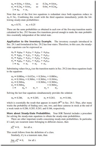
While calculating the n-step transition probabilities for both the weather and inventory examples in Sec. 29.3, we noted an interesting feature of these matrices. If n is large enough (n = 5 for the weather example and n = 8 for the inventory example), all the rows of the matrix have identical entries, so the probability that the system is in each state j no longer depends on the initial state of the system. In other words, there is a limiting prob- ability that the system will be in each state j after a large number of transitions, and this probability is independent of the initial state. These properties of the long-run behavior of finite-state Markov chains do, in fact, hold under relatively general conditions, as sum- marized below.
Thus, the probability of finding the process in a transient state after a large number of transitions tends to zero.
Expected Average Cost per Unit Time
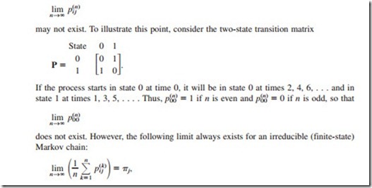
The preceding subsection dealt with irreducible finite-state Markov chains whose states were ergodic (recurrent and aperiodic). If the requirement that the states be aperiodic is relaxed, then the limit
where the TTj satisfy the steady-state equations given in the preceding subsection.
This result is important in computing the long-run average cost per unit time associated with a Markov chain. Suppose that a cost (or other penalty function) C(Xt) is incurred when the process is in state Xt at time t, for t = 0, 1, 2, . . . . Note that C(Xt) is a random variable that takes on any one of the values C(0), C(1), . . . , C(M) and that the function C(·) is independent of t. The expected average cost incurred over the first n periods is given by
Application to the Inventory Example. To illustrate, consider the inventory example introduced in Sec. 29.1, where the solution for the TTj was obtained in an earlier subsection. Suppose the camera store finds that a storage charge is being allocated for each camera remaining on the shelf at the end of the week. The cost is charged as follows:
Expected Average Cost per Unit Time for Complex Cost Functions
In the preceding subsection, the cost function was based solely on the state that the process is in at time t. In many important problems encountered in practice, the cost may also depend upon some other random variable.
For example, in the inventory example introduced in Sec. 29.1, suppose that the costs to be considered are the ordering cost and the penalty cost for unsatisfied demand (stor- age costs are so small they will be ignored). It is reasonable to assume that the number of cameras ordered to arrive at the beginning of week t depends only upon the state of the process Xt-1 (the number of cameras in stock) when the order is placed at the end of week t - 1. However, the cost of unsatisfied demand in week t will also depend upon the demand Dt. Therefore, the total cost (ordering cost plus cost of unsatisfied demand) for week t is a function of Xt-1 and Dt, that is, C(Xt-1, Dt).
Under the assumptions of this example, it can be shown that the (long-run) expected
The results of this subsection were presented only in terms of the inventory example. However, the (nonnumerical) results still hold for other problems as long as the following conditions are satisfied:


Comments
Post a Comment