MARKOV CHAINS:CONTINUOUS TIME MARKOV CHAINS
CONTINUOUS TIME MARKOV CHAINS
In all the previous sections, we assumed that the time parameter t was discrete (that is, t = 0, 1, 2, . . .). Such an assumption is suitable for many problems, but there are certain cases (such as for some queueing models considered in Chap. 17) where a continuous time parameter (call it t') is required, because the evolution of the process is being observed continuously over time. The definition of a Markov chain given in Sec. 29.2 also extends to such continuous processes. This section focuses on describing these “continuous time Markov chains” and their properties.
Steady-State Probabilities
Just as the transition probabilities for a discrete time Markov chain satisfy the Chapman- Kolmogorov equations, the continuous time transition probability function also satisfies these equations. Therefore, for any states i and j and nonnegative numbers t and s (0 < s < t),
The steady-state equation for state j has an intuitive interpretation. The left-hand side (wj qj) is the rate at which the process leaves state j, since wj is the (steady-state) proba- bility that the process is in state j and qj is the transition rate out of state j given that the process is in state j. Similarly, each term on the right-hand side (wi qij) is the rate at which the process enters state j from state i, since qij is the transition rate from state i to state j given that the process is in state i. By summing over all i -:: j, the entire right-hand side then gives the rate at which the process enters state j from any other state. The overall equation thereby states that the rate at which the process leaves state j must equal the rate at which the process enters state j. Thus, this equation is analogous to the conservation of flow equations encountered in many engineering and science courses.
Because each of the first M + 1 steady-state equations requires that two rates be in balance (equal), these equations sometimes are called the balance equations.
Example. A certain shop has two identical machines that are operated continuously except when they are broken down. Because they break down fairly frequently, the top- priority assignment for a full-time maintenance person is to repair them whenever needed.
The time required to repair a machine has an exponential distribution with a mean of -- day. Once the repair of a machine is completed, the time until the next breakdown of that machine has an exponential distribution with a mean of 1 day. These distributions are independent.
Define the random variable X(t') as X(t') = number of machines broken down at time t', so the possible values of X(t') are 0, 1, 2. Therefore, by letting the time parameter t' run continuously from time 0, the continuous time stochastic process {X(t'); t'> 0} gives the evolution of the number of machines broken down.
Because both the repair time and the time until a breakdown have exponential distributions, {X(t'); t'> 0} is a continuous time Markov chain5 with states 0, 1, 2. Consequently, we can use the steady-state equations given in the preceding subsection to find the steady-state probability distribution of the number of machines broken down. To do this, we need to determine all the transition rates, i.e., the qi and qij for i, j = 0, 1, 2.
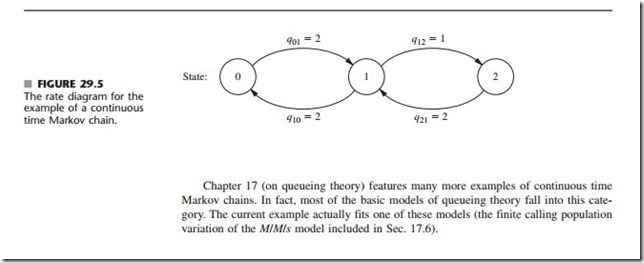
The state (number of machines broken down) increases by 1 when a breakdown occurs and decreases by 1 when a repair occurs. Since both breakdowns and repairs occur one at a time, q = 0 and q = 0. The expected repair time is 1 day, so the rate at which repairs are completed (when any machines are broken down) is 2 per day, which implies that q21 = 2 and q10 = 2. Similarly, the expected time until a particular operational machine breaks down is 1 day, so the rate at which it breaks down (when operational) is 1 per day, which implies that q12 = 1. During times when both machines are operational, breakdowns occur at the rate of 1 + 1 = 2 per day, so q01 = 2.
These transition rates are summarized in the rate diagram shown in Fig. 29.5. These rates now can be used to calculate the total transition rate out of each state.
Thus, in the long run, both machines will be broken down simultaneously 20 percent of the time, and one machine will be broken down another 40 percent of the time.
5Proving this fact requires the use of two properties of the exponential distribution discussed in Sec. 17.4 (lack of memory and the minimum of exponentials is exponential), since these properties imply that the Tij random variables introduced earlier do indeed have exponential distributions.


Comments
Post a Comment