MARKOV CHAINS:CHAPMAN-KOLMOGOROV EQUATIONS
CHAPMAN-KOLMOGOROV EQUATIONS
Section 29.2 introduced the n-step transition probability p(n). The following Chapman- Kolmogorov equations provide a method for computing these n-step transition probabilities:
3These equations also hold in a trivial sense when m = 0 or m = n, but m = 1, 2, . . . , n - 1 are the only interesting cases.
These equations point out that in going from state i to state j in n steps, the process
Thus, if the weather is in state 0 (dry) on a particular day, the probability of being in state 0 two days later is 0.76 and the probability of being in state 1 (rain) then is 0.24. Similarly, if the weather is in state 1 now, the probability of being in state 0 two days later is 0.72 whereas the probability of being in state 1 then is 0.28.
The probabilities of the state of the weather three, four, or five days into the future also can be read in the same way from the three-step, four-step, and five-step transition matrices calculated to three significant digits below.
Note that the five-step transition matrix has the interesting feature that the two rows have identical entries (after rounding to three significant digits). This reflects the fact that the probability of the weather being in a particular state is essentially independent of the state of the weather five days before. Thus, the probabilities in either row of this five-step transition matrix are referred to as the steady-state probabilities of this Markov chain.
We will expand further on the subject of the steady-state probabilities of a Markov chain, including how to derive them more directly, at the beginning of Sec. 29.5.
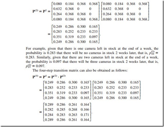
For example, given that there is one camera left in stock at the end of a week, the probability is 0.282 that there will be no cameras in stock 4 weeks later, that is, p(4) = 0.282. Similarly, given that there are two cameras left in stock at the end of a week, the probability is 0.171 that there will be three cameras in stock 4 weeks later, that is, p(4) = 0.171.
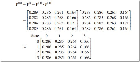
The transition probabilities for the number of cameras in stock 8 weeks from now can be read in the same way from the eight-step transition matrix calculated below.
Like the five-step transition matrix for the weather example, this matrix has the interesting feature that its rows have identical entries (after rounding). The reason once again is that probabilities in any row are the steady-state probabilities for this Markov chain, i.e., the probabilities of the state of the system after enough time has elapsed that the initial state is no longer relevant.
Your IOR Tutorial includes a procedure for calculating P(n) = Pn for any positive integer n :s 99.
Unconditional State Probabilities


Comments
Post a Comment