DYNAMIC PROGRAMMING:PROBABILISTIC DYNAMIC PROGRAMMING
PROBABILISTIC DYNAMIC PROGRAMMING
Probabilistic dynamic programming differs from deterministic dynamic programming in that the state at the next stage is not completely determined by the state and policy decision at the current stage. Rather, there is a probability distribution for what the next state will be. However, this probability distribution still is completely determined by the state
and policy decision at the current stage. The resulting basic structure for probabilistic dynamic programming is described diagrammatically in Fig. 11.10.
For the purposes of this diagram, we let S denote the number of possible states at stage n + 1 and label these states on the right side as 1, 2, . . . , S. The system goes to state i with probability pi (i = 1, 2, . . . , S) given state sn and decision xn at stage n. If the system goes to state i, Ci is the contribution of stage n to the objective function.
When Fig. 11.10 is expanded to include all the possible states and decisions at all the
stages, it is sometimes referred to as a decision tree. If the decision tree is not too large, it provides a useful way of summarizing the various possibilities.
Because of the probabilistic structure, the relationship between fn(sn, xn) and the f *n+1(sn+1) necessarily is somewhat more complicated than that for deterministic dy- namic programming. The precise form of this relationship will depend upon the form of the overall objective function.
To illustrate, suppose that the objective is to minimize the expected sum of the con- tributions from the individual stages. In this case, fn(sn, xn) represents the minimum ex- pected sum from stage n onward, given that the state and policy decision at stage n are sn and xn, respectively. Consequently,
EXAMPLE 5 Determining Reject Allowances
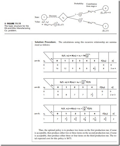
The HIT-AND-MISS MANUFACTURING COMPANY has received an order to supply one item of a particular type. However, the customer has specified such stringent quality requirements that the manufacturer may have to produce more than one item to obtain an item that is acceptable. The number of extra items produced in a production run is called the reject allowance. Including a reject allowance is common practice when producing for a custom order, and it seems advisable in this case.
The manufacturer estimates that each item of this type that is produced will be acceptable with probability -- and defective (without possibility for rework) with probability --.
Thus, the number of acceptable items produced in a lot of size L will have a binomial distribution; i.e., the probability of producing no acceptable items in such a lot is (1)L.
Marginal production costs for this product are estimated to be $100 per item (even if defective), and excess items are worthless. In addition, a setup cost of $300 must be in- curred whenever the production process is set up for this product, and a completely new setup at this same cost is required for each subsequent production run if a lengthy in- spection procedure reveals that a completed lot has not yielded an acceptable item. The manufacturer has time to make no more than three production runs. If an acceptable item has not been obtained by the end of the third production run, the cost to the manufacturer in lost sales income and penalty costs will be $1,600.
The objective is to determine the policy regarding the lot size (1 + reject allowance) for the required production run(s) that minimizes total expected cost for the manufacturer.
EXAMPLE 6 Winning in Las Vegas
An enterprising young statistician believes that she has developed a system for winning a popular Las Vegas game. Her colleagues do not believe that her system works, so they have made a large bet with her that if she starts with three chips, she will not have at least five chips after three plays of the game. Each play of the game involves betting any de- sired number of available chips and then either winning or losing this number of chips. The statistician believes that her system will give her a probability of 2 of winning a given play of the game.
Assuming the statistician is correct, we now use dynamic programming to determine her optimal policy regarding how many chips to bet (if any) at each of the three plays of the game. The decision at each play should take into account the results of earlier plays. The objective is to maximize the probability of winning her bet with her colleagues.
Formulation. The dynamic programming formulation for this problem is Stage n = nth play of game (n = 1, 2, 3), xn = number of chips to bet at stage n,
State sn = number of chips in hand to begin stage n.
This definition of the state is chosen because it provides the needed information about the current situation for making an optimal decision on how many chips to bet next.
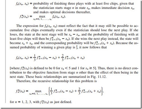
Because the objective is to maximize the probability that the statistician will win her bet, the objective function to be maximized at each stage must be the probability of fin- ishing the three plays with at least five chips. (Note that the value of ending with more than five chips is just the same as ending with exactly five, since the bet is won either way.) Therefore, fn(sn, xn) = probability of finishing three plays with at least five chips, given that the statistician starts stage n in state sn, makes immediate decision xn, and makes optimal decisions thereafter,
The expression for fn(sn, xn) must reflect the fact that it may still be possible to ac- cumulate five chips eventually even if the statistician should lose the next play. If she loses, the state at the next stage will be sn - xn, and the probability of finishing with at least five chips will then be f *n+1(sn - xn). If she wins the next play instead, the state will become sn + xn, and the corresponding probability will be f *n+1(sn + xn). Because the as- sumed probability of winning a given play is 2, it now follows that
This policy gives the statistician a probability of 20 of winning her bet with her colleagues.


Comments
Post a Comment