OTHER ALGORITHMS FOR LINEAR PROGRAMMING:PARAMETRIC LINEAR PROGRAMMING
PARAMETRIC LINEAR PROGRAMMING
At the end of Sec. 7.2 we mentioned that parametric linear programming provides an- other useful way for conducting sensitivity analysis systematically by gradually changing various model parameters simultaneously rather than changing them one at a time. We shall now present the algorithmic procedure, first for the case where the cj parameters are being changed and then where the bi parameters are varied.
Systematic Changes in the cj Parameters
For the case where the cj parameters are being changed, the objective function of the ordinary linear programming model

The values assigned to the aj may represent interesting simultaneous changes of the cj for systematic sensitivity analysis of the effect of increasing the magnitude of these changes. They may also be based on how the coefficients (e.g., unit profits) would change together with respect to some factor measured by 8. This factor might be uncontrollable, e.g., the state of the economy. However, it may also be under the control of the decision maker, e.g., the amount of personnel and equipment to shift from some of the activities to others.
For any given value of 8, the optimal solution of the corresponding linear program- ming problem can be obtained by the simplex method. This solution may have been ob- tained already for the original problem where 8 = 0. However, the objective is to find the optimal solution of the modified linear programming problem [maximize Z(8) subject to the original constraints] as a function of 8. Therefore, in the solution procedure you need to be able to determine when and how the optimal solution changes (if it does) as 8 in- creases from zero to any specified positive number.
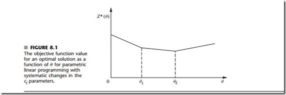
Figure 8.1 illustrates how Z*(8), the objective function value for the optimal solution (given 8), changes as 8 increases. In fact, Z*(8) always has this piecewise linear and convex3 form (see Prob. 8.2-7). The corresponding optimal solution changes (as 8 increases) just at the
3See Appendix 2 for a definition and discussion of convex functions.
values of 8 where the slope of the Z*(8) function changes. Thus, Fig. 8.1 depicts a problem where three different solutions are optimal for different values of 8, the first for 0 ::: 8 ::: 81, the second for 81 ::: 8 ::: 82, and the third for 8 2: 82. Because the value of each xj remains the same within each of these intervals for 8, the value of Z*(8) varies with 8 only because the coefficients of the xj are changing as a linear function of 8. The solution procedure is based directly upon the sensitivity analysis procedure for investigating changes in the cj parameters (Cases 2a and 3, Sec. 7.2). The only basic difference with parametric linear programming is that the changes now are expressed in terms of 8 rather than as specific numbers.
Therefore, after 8 is increased past 8 = , x4 would need to be the entering basic variable for another iteration of the simplex method, which takes us from the first tableau in Table
8.2 to the second tableau. Then 8 would be increased further until another coefficient goes negative, which occurs for the coefficient of x5 in the second tableau when 8 is increased past 8 = 5. Another iteration of the simplex method then takes us to the final tableau of Table 8.2. Increasing 8 further past 5 never leads to a negative coefficient in Eq. (0), so the procedure is completed.
Summary of the Parametric Linear Programming Procedure for Systematic Changes in the cj Parameters
1. Solve the problem with 8 = 0 by the simplex method.
2. Use the sensitivity analysis procedure (Cases 2a and 3, Sec. 7.2) to introduce the
!Jcj = aj8 changes into Eq. (0).
3. Increase 8 until one of the nonbasic variables has its coefficient in Eq. (0) go negative
(or until 8 has been increased as far as desired).
4. Use this variable as the entering basic variable for an iteration of the simplex method to find the new optimal solution. Return to step 3.
Note in Table 8.2 how the first two steps of this procedure lead to the first tableau and then steps 3 and 4 lead to the second tableau. Repeating steps 3 and 4 next leads to the final tableau.
Systematic Changes in the bi Parameters
For the case where the bi parameters change systematically, the one modification made in the original linear programming model is that bi is replaced by bi + ai8, for i = 1, 2, . . . , m, where the ai are given input constants. Thus, the problem becomes
The goal is to identify the optimal solution as a function of 8.
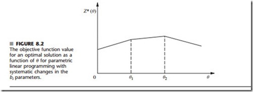
With this formulation, the corresponding objective function value Z*(8) always has the piecewise linear and concave4 form shown in Fig. 8.2. (See Prob. 8.2-8.) The set of basic variables in the optimal solution still changes (as 8 increases) only where the slope of Z*(8) changes. However, in contrast to the preceding case, the values of these variables now change as a (linear) function of 8 between the slope changes. The reason is that increasing 8 changes the right-hand sides in the initial set of equations, which then causes changes in the right-hand sides in the final set of equations, i.e., in the values of the final set of basic variables. Figure 8.2 depicts a problem with three sets of basic variables that are optimal for different values of 8, the first for 0 ::: 8 ::: 81, the second for 81 ::: 8 ::: 82, and the third for 8 2: 82. Within each of these intervals of 8, the value of Z*(8) varies with 8 despite the fixed coefficients cj because the xj values are changing.
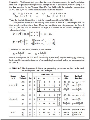
The following solution procedure summary is very similar to that just presented for systematic changes in the cj parameters. The reason is that changing the bi values is equiv- alent to changing the coefficients in the objective function of the dual model. Therefore, the procedure for the primal problem is exactly complementary to applying simultane- ously the procedure for systematic changes in the cj parameters to the dual problem. Consequently, the dual simplex method (see Sec. 8.1) now would be used to obtain each new optimal solution, and the applicable sensitivity analysis case (see Sec. 7.2) now is Case 1, but these differences are the only major differences.
Summary of the Parametric Linear Programming Procedure for Systematic Changes in the bi Parameters
1. Solve the problem with 8 = 0 by the simplex method.
2. Use the sensitivity analysis procedure (Case 1, Sec. 7.2) to introduce the £1bi = ai8 changes to the right side column.
3. Increase 8 until one of the basic variables has its value in the right side column go negative (or until 8 has been increased as far as desired).
4. Use this variable as the leaving basic variable for an iteration of the dual simplex method to find the new optimal solution. Return to step 3.
The Solved Examples section of the book’s website includes another example of the procedure for systematic changes in the bi parameters.


Comments
Post a Comment